One way to stop a 2D spaceship as fast as possible.

For a quite a while, I have wanted to try and create simple touch based interface for a 2D spaceship game. I want to allow the player to simply drag anywhere on the screen, and the spaceship moves to that position and direction in an efficient manner. Ideally the most efficient manner.

Spaceships in 2D games usually have one main engine that allows forward thrust, and some that allow rotation around the ships center of mass.

Moving from point A to B efficiently (in minimal time) is not trivial with such constraints, as changes to direction and thrust may have huge consequences for later possible movements due to inertia.

So instead of looking at the full A to B problem immediately, I wanted to look at something simpler first, namely to go from having velocity \(v_0\) and pointing in direction \(\theta_0\) to have 0 velocity as fast as possible.

The idea I use originally came from talking to a colleague, but something very similar sounding is mentioned in planning algorithms, though examples always seems to involve driftless systems. Anyway, my current approach involves these known quantities and assumptions:

  • \(a\) – Acceleration – The ship can only accelerate by a constant amount, and acceleration turns on and off instantly.
  • \(s\) – Turn speed – rotating the ship requires no acceleration, and the ship has constant rotation rate.
  • \(\theta_0\) – Initial orientation.
  • \(v_0\) – Initial velocity

These quantities allow me to find a legal, but very suboptimal way to stop. It simply involves to turn the ship to face its velocity vector, and then accelerate until it stops. Both the time needed to turn the ship \(t_a\) and the time \(t_m\) needed to turn and reverse the velocity are easy to calculate.

Turn until facing velocity and initiate burn at time \(t_a\). At \(t_m\) the ship has velocity 0.

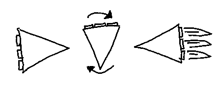
It is also easy to see that this is suboptimal, it would clearly be faster, to start burning some time before the turn is fully completed, but the question is when to start the burn.

To allow for this freedom in my model, I therefore introduce a third time variable \(t_s\). \(t_s\) is the time to start turning and accelerating at the same time. \(t_a\) now becomes the time when I stop turning and only accelerate.

Turn and initiate burn after \(t_s\) time, at \(t_a\) time only accelerate. At \(t_m\) the ship has velocity 0.

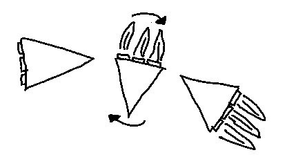
Given these intervals, two integrals describe how the velocity will change when \(t_s\), \(t_a\) and \(t_m\) vary.

$$ v_x = \int_{t_s}^{t_a} a\cos(\theta_0+st)dt + \int_{t_a}^{t_m} a\cos(\theta_0+st_a)dt $$

$$ v_y = \int_{t_s}^{t_a} a\sin(\theta_0+st)dt + \int_{t_a}^{t_m} a\sin(\theta_0+st_a)dt $$

This gives two constraints, that must hold for all solutions of this kind.

$$ 0 = v_{0x} + \int_{t_s}^{t_a} a\cos(\theta_0+st)dt + \int_{t_a}^{t_m} a\cos(\theta_0+st_a)dt $$

$$ 0 = v_{0y} + \int_{t_s}^{t_a} a\sin(\theta_0+st)dt + \int_{t_a}^{t_m} a\sin(\theta_0+st_a)dt $$

The most efficient solution to this problem, is the \(t_s\), \(t_a\) and \(t_m\) triplet with the lowest value for \(t_m\).

This information allows me to formulate this as a optimization problem.

Since I want to minimise \(t_m\), the objective function simply becomes \({t_m}^2\).

This is subject to the two equality constraints given.

Since the objective and constraints are non-linear, I plug i into Optizelle which is a framework for solving non-linear optimization problems.

The implementation can be found on github, it uses autograd, to calculate derivatives and hessians. This is an incredible time saver since calculating 9 combinations of partial derivatives would have been a major pain, not to mention having to recalculate them whenever I did something wrong.

Running the program with inputs \(a=2.0\), \(\theta_0=0\), \(v_0=[2,0]\) and \(s=\frac{\pi}{2}\) returns:

running-optizelle

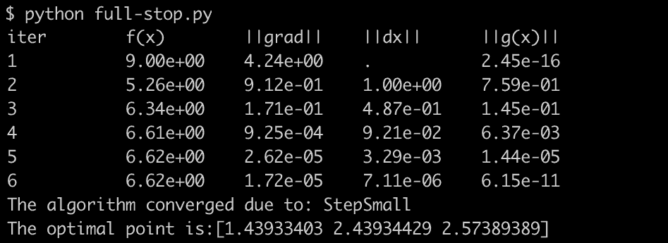
The optimal point vector contains the values for \(t_s\),\(t_a\) and \(t_m\). This means that for a ship with the given input, it should start turning immediately, then start the burn after approximately 1.43 seconds, stop turning and only accelerate at 2.43 and finally be at rest after 2.57 seconds, approximately 0.43 seconds faster then the naive version.

To test the result, I implemented a quick and dirty javascript program that simulates these choices and renders to a canvas:

Sometimes the ships end up drifting a bit after the simulation has finished. This is due to the discrete nature of the simulation not perfectly emulating the continuous solution (I do not integrate rotation analytically in the simulation). This could also have been a problem if I applied this style of planning to a game that did the same, from the simulation above it looks negligible though, which is great!

I am very happy with this result, it seems like it could work for the larger problem as well. The next step I’ll try, is to tackle some specific cases of moving from point A to B efficiently. For those cases there will be many more time variables involved, and possibly many constellations of safe initial starting points as well as possible freedoms to introduce in the model. It will be interesting to see how that works out.

Solving Get1000 continued…

In one of my previous posts, I laid out a plan to solve the Get 1000 game. It turns out that plan was wrong.

My expectiminimax based solution works well for a game with random elements and perfect information, but it is not very useful for a game with imperfect information. Get1000 is played simultaneously by the players, and the opponents choices are hidden until the end of the game.

This meant I had to go back to find a new strategy for solving the game. I decided to try and find the correct brute force way first, and then see if that could be made faster in some way.

Exploring brute force

A solution to the game involves finding a Nash equilibrium from all the pure strategies of the game. A brute force solution could be done by creating a matrix where all pure strategies are pitted against all the other pure strategies.

The full payoff matrix needed for a normal form brute force solution.

A strategy here refers to a function S \rightarrow Pl 
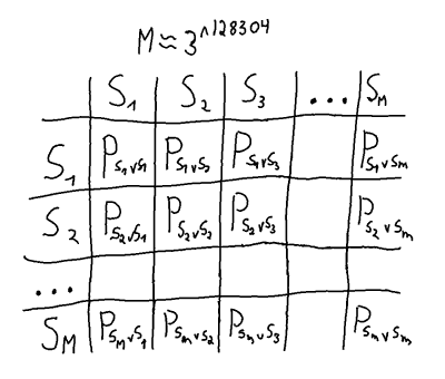
which given any game state S gives a Get1000 placement Pl. Below is an illustration of what i mean by a state. A state could also include the history (order of placement), which would increase the count a lot, but that is hopefully not needed for a solution.
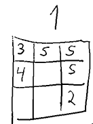
gamestate
A gamestate

A gamestate can be represented as the current number (in this case 1), the entries in hundres (7), tens (5) and ones (12) as well as the amount of free positions for hundreds (1), tens (2), ones(2).

The total amount of such states is 211248 but in at least 27648\cdot3 the choice is forced. This means there are at most. 211248 - 27648\cdot3 = 128304 relevant states, probably quite a bit fewer.


Each state has at most 3 choices, therefore there is an upper bound of M = 3^{128304} unique pure strategies.

This is of course not that helpful, since a 3^{128304}\times3^{128304} matrix is enormous, and for each cell in the matrix all possible 6^9 games would have to be played to find the payoff P for the pure strategy pairs. On top of that, the best mixed strategy would then have to be calculated.

Subgame perfection and backwards induction

Modeling this in normal form as above seemed to get me nowhere, I therefore turned to extensive form, and something called subgame-perfect nash equilibria, and backwards induction. In the normal form solution I need to look at all possible strategies. Using subgame perfection, I hoped to get away with only looking at a very small subset.

While this sounds straighforward in theory, I found it quite hard to figure out where my information sets are, and whether I could consider each choice node in Get1000 a subgame. After struggling for a while, I ended up with an extensive form structure looking like this. Players are P1 and P2, and “move by nature” is the dice roll.

Extensive form of a game with the same structure as Get1000. As players do their choices, the information sets get larger and larger. Since the “moves by nature” are known by all, they do not increase the information sets.

This structure means that only the roots of the tree are subgames, since all other nodes are part of larger information sets.

Attempting backwards induction

The above structure means that it is not practical to naively use subgame perfection and backwards induction to solve the game, but taking inspiration from it could still be useful to get a good strategy.

The algorithm for subgame perfection goes like this:

  1. Consider the final subgames (those with no further subgames), pick a Nash equilibrium as solution there.
  2. When considering the next subgames up the tree, the payoffs in the subgames already considered are used to create the payoff matrix.
  3. Iterate step 2 until the root node of the extensive form tree is reached.

To get something working, I pretend that the other player is at the same state as me always. This means I can only focus on the branches below that state. To keep memory in check i also recalculate payoffs instead of storing the result for each combination of states and games. The final algorithm I ended up with works like this:

  1. Consider the final subgames and pick a Nash equilibrium as solution.
  2. When looking at subgames higher up the tree, I use the choices (not payoffs) computed in 1, and use those choices to play out the game. Then I compare end results to get the payoff matrix for that subgame.
  3. As before, I iterate step 2 until I reach the root node.

This seems intuitively pretty reasonable.

Experimental results

The above method gives me a strategy that partly takes the imperfect information nature of the game into account. At many states it detected mixed strategies that had much higher payoffs compared to the pure versions. The strategies smashes all my previous best strategies by winning 1.75% more games.

The mixed strategy seems to play even more aggressively for results close to a 1000, and allowing heavy overshoot.

At this point, I was not really sure how to approach the game in a better way. In fact I was pretty ready to admin defeat for quite some time. Of course, immediately after i wrote that, I found this thesis, and this report.

Lots of new concepts to learn!

Attempting to solve Get 1000

For quite some time I have been trying to completely solve the Get 1000 game. More specifically I am trying to find the strategy in a 1 on 1 game of Get 1000 that maximises the chance to win.

Analysis of a game with one choice left. If I analyse this sub-game using expected value, I return the average of the distances to 1000. In this case 184 for strategy 1 (S1) and 107 for strategy 2 (S2). This is the wrong metric though, a better metric (if the goal is to win in a 1 on 1 game) is to count wins for each strategy. In this case 1 draw, 1 win for strategy 1 and 4 wins for strategy 2.

Solving for expected value rather then winning

My initial attempt at solving the game failed spectacularity, since I attempted to solve the game by minimising the average distance of the expected value to a 1000. This is an easy to compute strategy (using a sort of bottom up dynamic programming, where I start with the easy sub-games above, and calculate backwards to the top), but it is the wrong goal. This leads to a strategy minimising the distance to 1000 on average. This interestingly enough differs quite a lot from the goal I wanted to solve, which was to maximise the chance to win any 1 on 1 game.

The strategy that bases itself of minimising the distance to 1000 curiously has a big lump of results around a distance of 50, while the win based strategy has more games at distance of 0 and 100, as well as more games with very heavy over or undershoot.

Since Get 1000 is quite small I can calculate how much the two strategies differ by running all possible games. Above is the result of such a calculation. The two strategies draw 41.2% of the time, while the win based wins 30.8% and the distance based wins 28% of the time.

Trouble with situations where choices are equally good

After figuring out I had the wrong goal, I found a way to create a strategy based on wins rather than expected value (this is much harder to compute, even using the same bottom up approach, since it is not possible to collapse results to an average, and ever growing lists of results must be compared). These strategies I suspect are very close to optimal, but there was something funky going on.

There are situations in my calculations where two placement choices have equal amounts of winning sub-games. Initially I thought I could just set an order of preference of my choice for these, but the resulting strategies beat each other when applied to all possible games. If the order of preference did not matter this should not happen.

For the longest time I could not figure out why this happened. I started questioning whether the markov property held in the game (I am still not 100% sure it does).

Enlightenment

At this point I took a few steps back and looked at what would be the correct framework to model this game in. Turns out it can be modelled as a Markov Decision Process. That in itself was not very helpful, but it eventually got me reading about the expectiminimax algorithm. Expectiminimax is a version of minimax for games with chance involved. While I had to modify it a bit for a simultaneous turn game, I implemented it for some subproblems of get 1000, which I could calculate to the bottom.

While implementing it I realised that I again would have to code resolution for when two choices are equally good. While googling a bit about that, I randomly read about Nash Equilibrium, and mixed strategies. I was already aware of most of this, but it suddenly it dawned on me that my game might contain mixed strategies which could effect the outcome my expectiminimax calculation, and which I needed to take into account.

Wrong payoffs propagated in expectiminimax

Indeed, after searching for a bit, I found several cases where a mixed strategy is needed. The example below shows a expectiminimax situation where a mixed strategy is needed to get the best outcome.

A Get 1000 situation as solved by expectiminimax. The two games on top are the current situation for two players. To make a decision in expectiminimax we must then compute the payoff matrix by recursively analysing all possible sub-games until the end (returning expected payoffs), and then solve the payoff matrix. Using the solver here, this particular sub-game has the payoff of -98/39 (- means in favour of player 2). In this situation: Player 1 should play ones at ratio of 23/39 and hundreds 16/39, and player 2 should play tens at a ratio of 11/39 and hundreds 28/39.

While this exact situation will probably not arise assuming perfect play, the result still might matter since expectiminimax depends on all subgames propagating correct payoffs.

The road ahead

I need to include the support enumeration or theLemke-Howson algorithm for finding nash equlibrium in the placement situations that require it, and then I need to somehow make expectiminimax run for the full game. Currently I can only run expectiminimax (without Lemke-Howson) in reasonable time, for a game which has 6 placements left.

From AI: A modern approach, it seems A/B pruning can be used, but it seems to be less effective on games with chance. I guess it is worth a shot.

Gl hf to me…

Useful if caught in overly simplistic space combat

One of my favorite games, and by far the one I used the most time creating content for during my youth is Escape Velocity Nova. The Escape Velocity series are 2D space RPGs, which means there is lots of 2D space combat. In these types of games you typically have three main types of weapons, non-turreted, turreted and homing. Non-turreted and homing weapons are not really that complicated. The non-turreted fire in one direction (typically forward), while the homing weapon typically turns as hard as it can towards the target at maximum speed. Turreted weapons were always a puzzle to me though, they somehow knew where you would be, and fired to intercept your ship. I always wondered how this was done.

Some years later during a visualization class (on how to find intersections between geometric primitives) I was wondering if I could use geometric equations to figure out where a spaceship needs to aim its torpedo, if it knows the position and velocity of the target. Below is the solution I came up with. It assumes constant speed for the target and the torpedo.

The positions of something moving at constant speed, can be described by this equation where t denotes time, \vec{v} the current velocity and \vec{p_o} is the starting position. This restricts the position of the target to a line, where the position on the line is determined by t.

(1)   \begin{equation*} \vec{p} = \vec{p_o} + \vec{v}t \end{equation*}

For 2 dimensions this is:

(2)   \begin{equation*} \begin{pmatrix}p_x\\p_y\end{pmatrix} = \begin{pmatrix}p_{xo}\\p_{yo}\end{pmatrix} + \begin{pmatrix}v_x\\v_y\end{pmatrix}t \end{equation*}

The possible locations p of a constant speed (s) bullet fired from point c in any direction, are given by this equation, where again time is denoted by t. This restrict the possible positions to a circle which expands with time.

(3)   \begin{equation*} (st)^{2} = (\vec{p} - \vec{c})^{2} \end{equation*}

For 2 dimensions this is:

(4)   \begin{equation*} (st)^2 = (p_{x} - c_x)^2 + (p_{y} - c_y)^2 \end{equation*}

Now inserting the restrictions on p_x and p_y from 2 into 4 gives a polynomial that only depends on t:

(5)   \begin{equation*} (st)^2 = ((p_{xo}+v_xt) - c_x)^2 + ((p_{yo}+v_yt) - c_y)^2 \end{equation*}

Rearranging gives:

(6)   \begin{equation*} s^2t^2 = (p_{xo}-c_x + v_xt)^2 + (p_{yo}-c_y + v_yt)^2 \end{equation*}

Simplifying by setting constants i = p_{xo}-c_x and j = p_{yo} - c_y and moving towards standard form:

(7)   \begin{equation*} s^2t^2 = (i)^2 + 2iv_xt + v_x^2t^2 + (j)^2 + 2jv_yt + v_y^2t^2 \end{equation*}

Rearranging to standard form:

(8)   \begin{equation*} 0 = (v_y^2 + v_x^2 - s^2)t^2 + 2(iv_x + jv_y)t + (i)^2 + (j)^2 \end{equation*}

This is a quadratic equation, with coefficients:

(9)   \begin{equation*} a = v_y^2 + v_x^2 - s^2 \end{equation*}

(10)   \begin{equation*} b=2(iv_x + jv_y) \end{equation*}

(11)   \begin{equation*} c=i^2 + j^2 \end{equation*}

Solving the quadratic equation gives two solution for t, if an answer is positive and has no imaginary part, there is a solution to the problem.

Inserting a solution for t in equation 1 gives the x,y coordinates where the torpedo should be aimed, and where it will hit the target.

Below is an implementation of this, where the constant speed of the torpedo can be set. If there are two solutions, the smallest t is chosen. If there is no solution (typically because the target it too fast for the torpedo to catch) the torpedo is never launched.


canvas

As you can see in some cases, this does not take into account the size of the target, only the targets center. This can be remedied by using a representative selection of boundary points of the target instead, and firing if one of them would connect.

The solution does also not take into account how fast the target can change direction, or when the torpedo runs out of fuel. This can be handled by not firing if the time from the torpedo is fired to the impact is too long.

This method can also quite easily be expanded for an accelerating weapon or target. This will result in a higher degree polynomial though, which are mostly only possible to solve using numerical methods like Newtons’s method for example.

The van der Corput sequence

Lately I have been looking for a solid way to create a robust implementation moving a spaceship from one point to another. This turned out to be a hard problem, and led me to a lot of new literature, which included Steven M. LaValle’s Planning Algorithms. Randomly reading from it I found a small gem called the van der Corput sequence.

The van der Corput sequence is useful for sampling in an interval. LaValle discusses it as an option to random sampling within the context of sampling for planning algorithms. I had thought about similar issues in the context of root finding, where I always wondered how to predictably generate a sequence that would distribute samples evenly over an interval, as well as do so in a manner that would not “favor” parts of the interval over others.

One naive way to sample over an interval, is to split the interval in X pieces and do the samples in order. If X is 8 and this method is used the interval would be explored as shown to the left in the figure below (clearly this means the the early parts of the interval will be explored first). Using the van der Corput sequence would result in exploration as seen on the right (which explores the interval much more evenly).

Van der Corput
Naive sampling on the left. Van der Corput sampling on the right. Grey circles show performed samples.

Generating the van der Corput sequence is surprisingly simple and elegant, just flip the bits of the naive sequence as seen in the binary column above. I find this very peculiar, since mirrored donkeys do not normally turn into cheetahs.

The great properties of this sequence is that whenever you end it, it will have explored the interval pretty evenly. A second nice property is that you can easily continue the sequence beyond an initial size, by creating the naive sequence at the position you want to start from, and keep reversing the results.

This method will definitely go into my toolbox of things to consider whenever I am thinking about using random sampling.

Comments and HTML5 scatterplots

To try and learn some Javascript and use of the HTML5 canvas, I decided to make a visualization tool. After some googling I decided on scatterplots that allow linking and brushing. My idea was to allow such plots to easily be added to any webpage or blog. At the moment they only work well in Webkit based browsers (Chrome, Safari) though.

If you are not familiar with visualization lingo, brushing basically means that you can select datapoints in some fashion. Linking means selections are propagated across two linked views. So if I select some datapoints in one plot the same datapoints are selected in a linked plot. Below is an example of the canvas based scatterplot implementation I ended up with. To try the linking and brushing scroll down to here.


canvas

As you might have understood from the axis names, instead of generating a dataset, I wanted to apply this to some real world data. The idea was inspired by “kommentarfeltdugnad”, which aim to not let extremism run unchallengde in public newspaper discussions. I have a hard time finding anything I want to do less then argue in a newspaper comment section, instead i figured studying the people doing this would be more interesting. Using visualization for this was inspired by Correll et al’s excellent paper on text visualization. If possible I would like to implement several more of their approaches later on.

Kommentarfeltdugnad also got me thinking about alternative approaches to discussion and forum moderation, especially wondering if it is possible to profile writers over time based on their writing, and ban or even hellban users which pass a certain threshold of badly argued or impossible to decipher posts.

The dataset I’m using in this post was derived from this article due to the amount of comments. All HTML is stripped away and descriptive parameters derived from the remaining comment data.

The aim of the initial exploration of this dataset is to see if it is possible to connect some derived parameters, and possibly tie these to certain usage of some words. You are of course compelled to explore the datasets yourself using the interactive scatterplots below.

I quickly figured out that a large percentage of comments were to short to make out any meaningful statistic. I decided that comments below 50 words were not to be included. Even though 50 is quite arbitrary and decimal oriented.

From the remaining posts I derived several parameters describing each post:

  • Percent of capitals.
  • Percent of punctuation.
  • Amount of words.
  • Percentage of occurrences of specific words (islam, muslim, sosialism, …).
  • Letters in post.

Initially I thought I would start with something obvious as a test of my data data. I think it reasonable to assume a very strong correlation between the amount of letters and words in a post. This can be seen in this plot.

Less obvious is whether there is a correlation between the percent of capitals and an excessive amount of punctuation in a post. Is it so that excessive capitals typers are more likely to either forgo or misuse punctuation?

Even more hypothetical is whether there is a correlation between mentions of islam or muslims and excessive use of capitals?

Below three scatterplots are linked together, with the first showing percentage of capitals and punctuation, the second showing word count and letters in post, the third shows percentage of capitals and percentage of words that are (islam/muslim). This allows for exploration of some of the questions above, as well as some other questions.


canvas2

canvas3

canvas4

There seems to be a small correlation between the amount of capitals and punctuation in a post. It would be very interesting to compare this dataset to a dataset with properly typed text. I also think that punctuation is very broad, and just focusing on exclamation and question marks might also be interesting.

The percentage of capitals and occurrences of islam seems not really related, though curiously, very long posts with a high amount of capitals do not seem to mention islam for some reason.

I guess that concludes my very superficial analysis of this dataset. Feel free to do whatever with the dataset, and once cleaned up I’ll link a zip with the JS source for convenience. My next posts will detail how to scrape the data, and how to add scatterplots to your own webpage or wordpress blog.


Finding matrix position from vector address

I have a symmetric matrix, which is stored as a vector containing only the needed elements. Is there an easy way to go from vector address to positions in the matrix?

The same operation on a square matrix stored in this way is done by:

(1)   \begin{equation*} x = v \mod{n} \end{equation*}

and

(2)   \begin{equation*} y = \frac{v}{m} \end{equation*}

Where v is the position in the vector, and m and n matrix columns and rows. This also conveniently reduces to bit shifts and masking if m and n are powers of 2. Operations are of course Integer operations.

My question is whether there exists a similar simple operation on a vector containing just one of the parts of a symmetric matrix.


Example of problem
Symmetric matrix stored in vector, not necessarily the best way to store it but one of many possibilities.

One opportunity is to use that the amount of elements needed to store a symmetric matrix is given by:

(3)   \begin{equation*} \frac{n(n+1)}{2} \end{equation*}

Using this one can iteratively search over n until the vector address is contained in the current block of inspected data. Then the remaining elements along with the amount of removed elements give the position. The problem is that this is n operations in a linear search, or log(n) operations if binary search is used.

so I’m wondering if there is an easier way to do this. Basically what I want is a very quick algorithm from vector position to matrix position.

Possibly useful observations are that the result from. n(n+1)/2 can always be divided by the odd component part of n and n+1, as well as the even component divided by two.

Also the resulting triangle can be divided into a structured amount s of square areas of values w:

(4)   \begin{equation*} s = 2^i \end{equation*}

(5)   \begin{equation*} w = \lfloor\frac{(n+2^i)}{2^{(i+1)}}^2\rfloor \end{equation*}

Where i is the squares where 0 is the largest square, and larger i gives the next smaller one. n is from the original matrix m and n. When the result is zero no more squares are needed to describe the area.

How this can be turned into a storage and addressing scheme, I do not know, and I wonder if there is no faster way (the binary search) to recover a position (without storing them beforehand) when something is stored in this manner?

Note that I’m not discussing packing and unpacking the entire matrix here (which would be O(n) using the linear search method from above), but finding the position of a single element from its position in the vector.